
This is a method for fuzzy search (extraction) with the FILTER function.
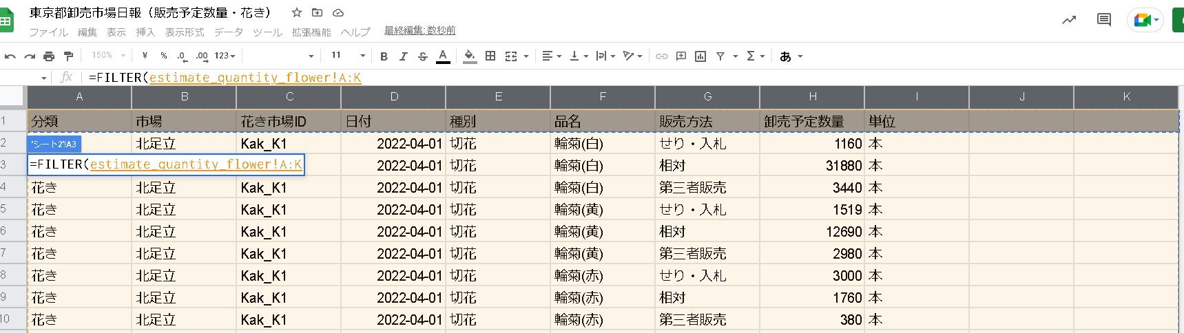
What is the FILTER function?
You can use the FILTER function to extract the result of a specific condition from within a range.
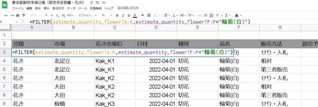
=FILTER(array, contains, [if empty])By using the FILTER function of Google Sheets, you can extract the result of the specified value from the table.
I was able to extract the ring chrysanthemum (white) in row F.
Is fuzzy search not possible with the FILTER function?
Even if you try to do a fuzzy search with this filter function, the result will not be returned as it is. Is it possible with asterisk? And even if I try, it will return an error (no matches).
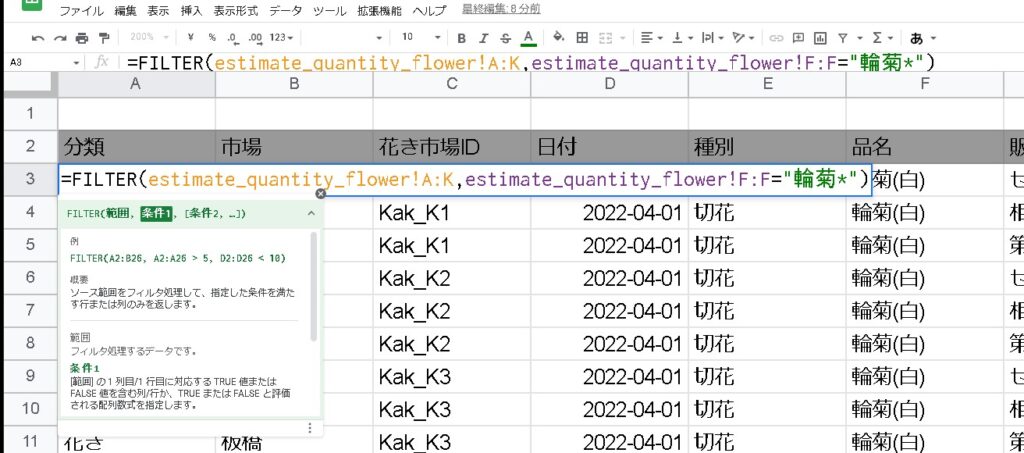
=FILTER(estimate_quantity_flower!A:K,estimate_quantity_flower!F:F="輪菊*")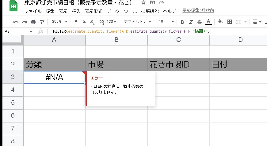
In this case, it is a method to realize a fuzzy search.
Combining FIND functions
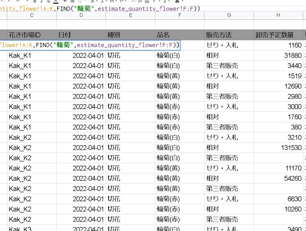
Now combine the FIND function.
=FILTER(estimate_quantity_flower!A:K,FIND("輪菊",estimate_quantity_flower!F:F))FIND 関数は、指定した文字列 (“輪菊”) が estimate_quantity_flower シートの F 列に存在する位置を返します。
FIND("輪菊",estimate_quantity_flower!F:F)Because the FIND function returns an error if the specified string is not found, this entire formula will only filter rows that contain the string “Ringiku” in column F.
As a result, this formula returns only rows in columns A through K of the estimate_quantity_flower sheet that contain the string “Ringiku” in column F.
The fuzzy search returned some results!
summary
Combining the FIND function with the FILTER function changed it to “contains”.
Why is the return value of the FIND function like this…? is a mystery at the moment, but by combining the FILTER function and the FIND function, it is possible to extract fuzzy filters.
Please refer to it.