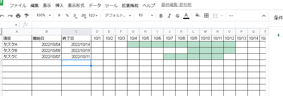
If you want to fill cells that correspond to dates from the start date, you can create a condition for the case where the value is less than or equal to the start date, such as “=$B2<=D$1”.
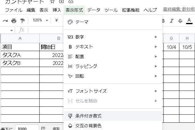
Apply to range * Range is bottom row of rightmost column
D2:BT10=$B2<=D$1If you specify the range starting from the top left of the table (below the date) and specify it with a relative reference, the cells from the start date onwards will be filled with the color as shown below.
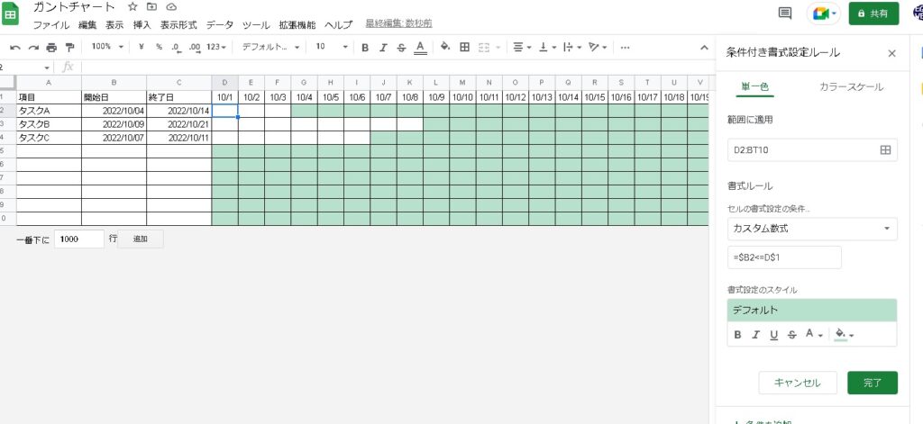
Filled.
Fill cells that correspond to dates “until the end date”
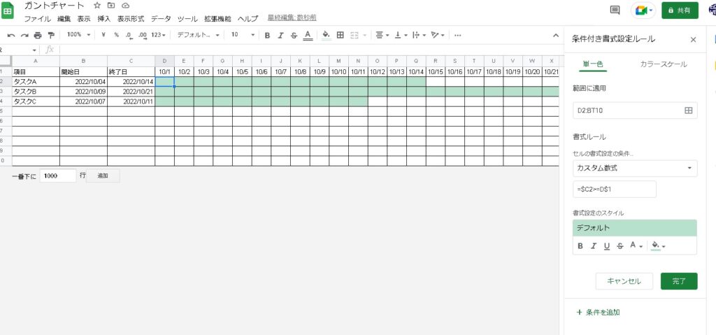
If you leave it like this, only the results from the start date will be displayed, so you will also fill the colors until the end date.
Apply to range * Range is bottom row of rightmost column
D2:BT10=$C2>=D$1This creates a conditional format with a compound reference up to the end date.
Concatenate with the AND function
Next, combine the above two with the AND function.
=AND($B2<=D$1,$C2>=D$1)The start date and end date have been filled in!
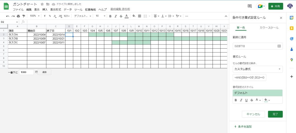
The cells from the start date to the end date have been filled in.

Summary
By using conditional formatting, I was able to create a Gantt chart.
It’s simple, but depending on how you use it, I think it can be useful. Please refer to it.

